Understanding JWST Pointing

In this notebook, we will go over a few concepts related to JWST pointing that can be confusing when we start looking at it in more details. Or at least concepts that were confusing for me when I did!

In this tutorial, we will use a NIRCam image from program GO 2473. This program aimed to search for companions around Y-type brown dwarfs at close and wide separations. This means that the images have a wide field of view, but we care primary about a single point source.

NIRCam is also a good instrument to play with since it has a long-wavelength and a short-wavelength channel, meaning that we can explore the connection between pointing in the two channels later on.

Downloading an observation

Let us first download the observation.

from pathlib import Path
from astroquery.mast import Observations

data_dir = Path("data")
program_dir = "02473"

filename = Path("jw02473064001_04101_00001_nrcblong_cal.fits")
uri = f"mast:JWST/product/{filename}"

filepath = data_dir / program_dir / filename
filepath.parent.mkdir(exist_ok=True, parents=True)
_ = Observations.download_file(uri, local_path=filepath)

INFO: Found cached file data/02473/jw02473064001_04101_00001_nrcblong_cal.fits with expected size 117573120. [astroquery.query]

Previewing the image

Let us first take a look at the full science image just to understand the data we are working with.

from astropy.io import fits

with fits.open(filepath) as hdul:
    hdr = hdul[0].header
    img = hdul[1].data
    sci_hdr = hdul[1].header

from matplotlib import rcParams
import matplotlib.pyplot as plt

rcParams["image.origin"] = "lower"

plt.imshow(img, norm="symlog")
plt.xlabel("X [pixel]")
plt.ylabel("Y [pixel]")
plt.show()

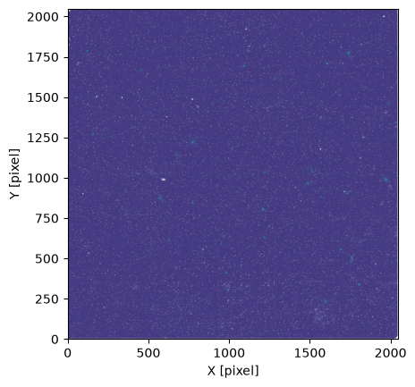
As explained above, this is a wide field image and it’s not easy to spot the companion. We identified it manually using the short and long-wavelength data to spot a very red point source and found it at (1211, 805) in pixel coordinates.

Let us see where this falls on the detector.

x_manual, y_manual = 1211, 805
plt.imshow(img, norm="symlog")
plt.plot(x_manual, y_manual, "r*", label="Manual position")
plt.xlabel("X [pixel]")
plt.ylabel("Y [pixel]")
plt.show()

It is hard to see if there is actually a point source there, so let us zoom in.

from jwpoint.plot import zoom_plot

zoom_plot(img, x_manual, y_manual, size=64, show_mask=False)
plt.xlabel("X [pixel]")
plt.ylabel("Y [pixel]")
plt.show()

Great, seems like we did find our target! Let us now use this data to understand the JWST pointing.

Finding the science target using pointing information

In the Getting started tutorial, we saw that we can predict the pointing position using the get_pointing_position() function.

from jwpoint.pointing import get_pointing_position

x_point, y_point = get_pointing_position(hdr["XOFFSET"], hdr["YOFFSET"], filepath)
print(f"Pointing position: ({x_point:.2f}, {y_point:.2f})")

Pointing position: (1234.81, 773.98)

One might note that this is quite off from the manual position of (1211, 805). Several factors can play into this. Here the main one is proper motion uncertainty at the time of planning the observations. However, we can see that the two points do not fall too far from each other when overplotting them on the image.

plt.imshow(img, norm="symlog")
plt.plot(x_manual, y_manual, "r*", label="Manual position")
plt.plot(x_point, y_point, "k+", label="Pointing position")
plt.xlabel("X [pixel]")
plt.ylabel("Y [pixel]")
plt.show()

This just means that if we do a zoomed-in plot, we might need to use a slightly larger size to make sure the full source is included…

zoom_plot(img, int(x_point), int(y_point), size=120, show_mask=False)
plt.xlabel("X [pixel]")
plt.ylabel("Y [pixel]")
plt.show()

This is not ideal but most piplines that need a small cutout will provide a re-center or cropping step to handle this. Otherwise just use jwpoint as a first pass to find the target and determine a more precise position.

A note on offsets and reference positions

At this point, it is probably worth explaining get_pointing_position() in a bit more detail. First of all, it takes as arguments the X and Y offsets from the header. Let’s see what the header comments tell us about these values:

print(hdr.cards["XOFFSET"])
print(hdr.cards["YOFFSET"])

XOFFSET =    19.10005767104914 / [arcsec] X offset in SI ideal coordinate frame 
YOFFSET =  -11.099997869097717 / [arcsec] Y offset in SI ideal coordinate frame 

The science instrument ideal coordinates are used for dithers and pointing offsets and aligned with the detector pixel coordinates.

The XOFFSET and YOFFSET keys describe the pointing offsets applied from the reference position for a given aperture. Apertures define detector regions and reference ponts. The NIRCam Apertures JDocs page describes this in more details and provides the reference point for each aperture. The aperture reference points are stored in jwpoint and can easily be accessed for all supported apertures:

from jwpoint.pointing import V2V3_REF_DICT
V2V3_REF_DICT

{'NRCBS_FULL': (-83.63, -495.98),
 'NRCB5_FULLP': (-133.181, -446.804),
 'NRCB5_SUB400P': (-148.665, -432.148)}

The aperture used for our observation can be retrieved from the header:

print(hdr.cards["PPS_APER"])

PPS_APER= 'NRCBS_FULL'         / original AperName supplied by PPS              

Note that the aperture coordinates are defined in the V2-V3 observatory coordinates. This is not the same as the X-Y detector pixel coordinates. This is why a file is required as the third argument to get_pointing_position(): it is used to convert between X-Y and V2-V3 coordinates.

Note that the header of the SCI extension has some “reference point” fields:

print(sci_hdr.cards["CRPIX1"])
print(sci_hdr.cards["CRPIX2"])
print(sci_hdr.cards["V2_REF"])
print(sci_hdr.cards["V3_REF"])

CRPIX1  =               1024.5 / Axis 1 pixel coordinate of ref point, 1-indexed
CRPIX2  =               1024.5 / Axis 2 pixel coordinate of ref point, 1-indexed
V2_REF  =           -89.402822 / [arcsec] Telescope V2 coord of reference point 
V3_REF  =          -491.360126 / [arcsec] Telescope V3 coord of reference point 

These typically point to the center of the detector and are not equivalent to the aperture reference point. Therefore, they should not be used for pointing calculations.

How jwpoint handles coordinate systems

As explained above, there are two coordinate systems we are primarily concerned with:

• The X-Y science instrument ideal coordinates

• The V2-V3 observatory coordinates

To convert between these systems, we need a World Coordinate System (WCS). This is added to the data products after stage 1 processing by the JWST pipeline, so we can extract it from the file metadata.

Internally, jwpoint does this by opening files as “data model” objects used in the jwst pipeline.

from jwst import datamodels

model = datamodels.open(filepath)

To convert between arcsec and pixels, we need the pixel scale of the detector

from jwpoint.pointing import PSCALE_DICT
detector = model.meta.instrument.detector
print(f"Detector: {detector}")
pscale = PSCALE_DICT[detector]
print(f"Pixel scale: {pscale} arcsec")

Detector: NRCBLONG
Pixel scale: 0.063 arcsec

We can also get the aperture and, in turn the reference point:

aperture = model.meta.aperture.pps_name
print(f"Aperture: {aperture}")
v2_ref, v3_ref = V2V3_REF_DICT[aperture]
print(f"V2-V3 reference position: {v2_ref, v3_ref}")

Aperture: NRCBS_FULL
V2-V3 reference position: (-83.63, -495.98)

The model’s WCS provides a transform() methods to transform between reference frames. The available reference frames are:

model.meta.wcs.available_frames

['detector', 'v2v3', 'v2v3vacorr', 'world']

If we want the reference position in pixel, we can convert it like this:

x_ref, y_ref = model.meta.wcs.transform("v2v3", "detector", v2_ref, v3_ref)

To apply the offset, we need to extract it from the header, convert it from arcsec to pixels and apply it to the pixel reference position:

x_off = hdr["XOFFSET"] / pscale
y_off = hdr["YOFFSET"] / pscale
x_point_demo = x_ref + x_off
y_point_demo = y_ref + y_off
print(f"Pointing position: ({x_point:.2f}, {y_point:.2f})")
print(f"Pointing position: ({x_point_demo:.2f}, {y_point_demo:.2f})")

Pointing position: (1234.81, 773.98)
Pointing position: (1234.81, 773.98)

As we can see, we just reproduced the exact result from get_pointing_position() with the above cells.

Note that get_pointing_position can apply the offset in two ways, determined by the offset_frame argument:

• detector: convert the reference point to x-y detector position and apply the offset in pixels

• v2v3: apply the offset directly to V2-V3 coordinates in arcseconds and only then transform to pixel coordinates

x_point_v2v3, y_point_v2v3 = get_pointing_position(hdr["XOFFSET"], hdr["YOFFSET"], filepath, offset_frame="v2v3")
print(f"Pointing for X-Y offset: ({x_point:.2f}, {y_point:.2f})")
print(f"Pointing for V2-V3 offset: ({x_point_v2v3:.2f}, {y_point_v2v3:.2f})")

Pointing for X-Y offset: (1234.81, 773.98)
Pointing for V2-V3 offset: (1234.66, 773.94)

As shown above, the two methods almost give the same result. We recommend just using the default offset_frame="detector" for consistency.

Understanding dither positions

from mastodown import query_obs, download_products

products = query_obs(
    programs="02473",
    calib_level=2,
    product_subgroup="CAL",
    extension="fits",
    target_name=hdr["TARGPROP"],
    filters="F480M",
)
products

INFO: 5 of 86 products were duplicates. Only returning 81 unique product(s). [astroquery.mast.utils]
INFO: To return all products, use `Observations.get_product_list` [astroquery.mast.observations]

	target_name	obsID	obs_collection	dataproduct_type	obs_id	description	type	dataURI	productType	productGroupDescription	...	productDocumentationURL	project	prvversion	proposal_id	productFilename	size	parent_obsid	dataRights	calib_level	filters
0	WISE-1206+84	118051331	JWST	image	jw02473064001_04101_00001_nrcblong	exposure (L2b): 2D calibrated exposure average...	S	mast:JWST/product/jw02473064001_04101_00001_nr...	SCIENCE	NaN	...	NaN	CALJWST	2.0.1	2473	jw02473064001_04101_00001_nrcblong_cal.fits	117573120	118051355	PUBLIC	2	F480M
1	WISE-1206+84	118051312	JWST	image	jw02473064001_04101_00002_nrcblong	exposure (L2b): 2D calibrated exposure average...	S	mast:JWST/product/jw02473064001_04101_00002_nr...	SCIENCE	NaN	...	NaN	CALJWST	2.0.1	2473	jw02473064001_04101_00002_nrcblong_cal.fits	117573120	118051355	PUBLIC	2	F480M
2	WISE-1206+84	118036322	JWST	image	jw02473064001_04101_00003_nrcblong	exposure (L2b): 2D calibrated exposure average...	S	mast:JWST/product/jw02473064001_04101_00003_nr...	SCIENCE	NaN	...	NaN	CALJWST	2.0.1	2473	jw02473064001_04101_00003_nrcblong_cal.fits	117573120	118051355	PUBLIC	2	F480M
3	WISE-1206+84	118038295	JWST	image	jw02473064001_04101_00004_nrcblong	exposure (L2b): 2D calibrated exposure average...	S	mast:JWST/product/jw02473064001_04101_00004_nr...	SCIENCE	NaN	...	NaN	CALJWST	2.0.1	2473	jw02473064001_04101_00004_nrcblong_cal.fits	117573120	118051355	PUBLIC	2	F480M
4	WISE-1206+84	118051318	JWST	image	jw02473064001_04101_00005_nrcblong	exposure (L2b): 2D calibrated exposure average...	S	mast:JWST/product/jw02473064001_04101_00005_nr...	SCIENCE	NaN	...	NaN	CALJWST	2.0.1	2473	jw02473064001_04101_00005_nrcblong_cal.fits	117573120	118051355	PUBLIC	2	F480M

5 rows × 21 columns

downloaded_products = download_products(products, download_dir=data_dir)

xoffsets = []
yoffsets = []
patt_nums = []
for path in downloaded_products.local_path:
    with fits.open(path) as hdul:
        hdr = hdul[0].header
    xoffsets.append(hdr["XOFFSET"])
    yoffsets.append(hdr["YOFFSET"])
    patt_nums.append(hdr["PATT_NUM"])

downloaded_products["XOFFSET"] = xoffsets
downloaded_products["YOFFSET"] = yoffsets
downloaded_products["PATT_NUM"] = patt_nums

for i, row in downloaded_products.iterrows():
    plt.scatter(row.XOFFSET, row.YOFFSET, marker=f"${row.PATT_NUM}$", color="C0")
plt.xlabel("X Ideal [arcsec]")
plt.xlabel("Y Ideal [arcsec]")
plt.title("Dither positions from the header")
plt.show()

from jwpoint.dithers import get_dither_info

pattern = hdr["PATTTYPE"]
dither_df = get_dither_info(pattern, n_dithers=len(downloaded_products))

for i, row in dither_df.iterrows():
    plt.scatter(row.x, row.y, marker=f"${i+1}$", color="C0")
plt.xlabel("X Ideal [arcsec]")
plt.xlabel("Y Ideal [arcsec]")
plt.title("Dither positions from JDocs")
plt.show()

Let us now compare them on the same plot.

from matplotlib.lines import Line2D

for i, row in downloaded_products.iterrows():
    plt.scatter(row.XOFFSET, row.YOFFSET, marker=f"${row.PATT_NUM}$", color="C1")
for i, row in dither_df.iterrows():
    plt.scatter(row.x, row.y, marker=f"${i+1}$", color="C0")
plt.xlabel("X Ideal [arcsec]")
plt.xlabel("Y Ideal [arcsec]")
plt.title("Dither positions from the header vs from JDocs")
plt.legend(
    handles=[
        Line2D([], [], label="header"),
        Line2D([], [], label="docs"),
    ],
    handlelength=0,
    handletextpad=0,
    labelcolor=["C1", "C0"],
)
plt.show()

As we can see, the shape and scale of the pattern is the same, but they are offset. This is because the offsets from the header also include the required pointing offset, which for this observation was (-22, 8) arcsec.

Visualizing dithers

jwpoint includes a utility function to show all dithers. It will first display the dithers on the full frame image and then a zoom on each dither. The former is useful to see where the dithers fall (e.g. are they close to an edge?), while the latter helps identify bad pixels or other detector cosmetics.

from jwpoint.plot import plot_dithers

x_all = []
y_all = []
for i, row in downloaded_products.iterrows():
    x, y = get_pointing_position(row.XOFFSET, row.YOFFSET, row.local_path)
    x_all.append(x)
    y_all.append(y)

plot_dithers(
    img,
    x_all,
    y_all,
    size=120,
    show_mask=False,
)
plt.show()

We could also disable the full frame image and show the DQ map

plot_dithers(
    img,
    x_all,
    y_all,
    size=120,
    full_frame=False,
    show_mask=True,
)
plt.show()

Finally, if we have a PSF with the same size as size, we can display it under the DQ mask to see where bad pixels would fall on a point source.

hs = 120 // 2
psf = img[y_manual - hs: y_manual + hs, x_manual - hs: x_manual + hs]

plot_dithers(
    img,
    x_all,
    y_all,
    size=120,
    full_frame=False,
    psf=psf,
)
plt.show()

Looking at the short-wavelength channel

For NIRCam imaging, observations are taken in both the short and long-wavelength (SW and LW) channels. So far, we have only looked at LW observations (NRCBLONG detector in the F480M filter). The SW channel splits the image between four detectors (NRCB1, NRCB2, NRCB3, NRCB4). jwpoint provides functionality to determine:

• On which SW detector does the LW position fall

• The SW detector coordinates based on the LW ones

First, using the manually determined position and the LW subarray, we determine the SW detector

import jwpoint.utils as ut

detector_sw = ut.get_sw_detector(x_manual, y_manual, hdr["SUBARRAY"])
detector_sw

'nrcb2'

To download the SW file, we simply replace the LW nrcblong detector with the SW detector in the filename. There is a utility function do figure out the SW detector and download the file automatically from a LW file.

filepath_sw = ut.download_sw_file(filepath, x_manual, y_manual)

INFO: Found cached file data/02473/jw02473064001_04101_00001_nrcb2_cal.fits with expected size 117573120. [astroquery.query]

with fits.open(filepath_sw) as hdul_sw:
    hdr_sw = hdul_sw[0].header
    img_sw = hdul_sw[1].data

We can then use the two files to convert the LW position to a SW position.

from jwpoint.pointing import long_to_short

x_manual_sw, y_manual_sw = long_to_short(x_manual, y_manual, filepath, filepath_sw)

Let’s see where this falls on the detectors.

fig, axs = plt.subplots(1, 2, figsize=(10, 5))
ax_lw, ax_sw = axs
ax_lw.imshow(img, norm="symlog")
ax_lw.plot(x_manual, y_manual, "r*", label="Manual position")
ax_lw.set_xlabel("X [pixel]")
ax_lw.set_ylabel("Y [pixel]")

ax_sw.imshow(img_sw, norm="symlog")
ax_sw.plot(x_manual_sw, y_manual_sw, "r*")
ax_sw.set_xlabel("X [pixel]")
ax_sw.set_ylabel("Y [pixel]")
plt.show()

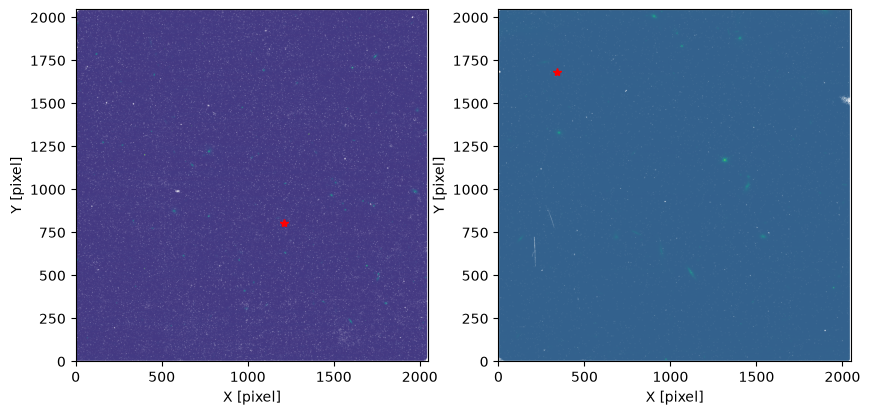
This makes sense since NRCB2 is at the bottom right if the field of view (see JDocs). But again, a zoomed plot would be more helpful. Let us check the point source side-by-side in the two filters.

fig, axs = plt.subplots(1, 2, figsize=(10, 5))
ax_lw, ax_sw = axs
pscale_sw = PSCALE_DICT[hdr_sw["DETECTOR"]]
size_factor = pscale_sw / pscale
zoom_plot(img, x_manual, y_manual, size=64, axs=ax_lw, show_mask=False)
zoom_plot(img_sw, int(x_manual_sw), int(y_manual_sw), size=int(64 * size_factor), axs=ax_sw, show_mask=False)
ax_lw.set_title("Long-wavelength")
ax_lw.set_xlabel("X [pixel]")
ax_lw.set_ylabel("Y [pixel]")
ax_sw.set_title("Short-wavelength")
ax_sw.set_xlabel("X [pixel]")
ax_sw.set_ylabel("Y [pixel]")
plt.show()